Sampling Distributions - AP Statistics
Card 0 of 20
Assume you have taken 100 samples of size 64 each from a population. The population variance is 49.
What is the standard deviation of each (and every) sample mean?
Assume you have taken 100 samples of size 64 each from a population. The population variance is 49.
What is the standard deviation of each (and every) sample mean?
The population standard deviation =

The sample mean standard deviation =

The population standard deviation =
The sample mean standard deviation =
Compare your answer with the correct one above
A random variable has an average of  with a standard deviation of
  . What is the probability that out of the sample set the variable is less than
  . The sample set is
  . Round your answer to three decimal places.
A random variable has an average of
There are two keys here. One, we have a large sample size since  , meaning we can use the Central Limit Theorem even if points per game is not normally distributed.
Our  -score thus becomes...
}{\sqrt{n} \cdot \sigma}")
where  is the specified points or less needed this season,
 is the average points per game of the previous season,
 is the standard deivation of the previous season,
and  is the number of games.
}{\sqrt{80} \cdot 5}=0.8944")
 = 0.8133")
There are two keys here. One, we have a large sample size since
Our
where
and
Compare your answer with the correct one above
Reaction times in a population of people have a standard deviation of  milliseconds. How large must a sample size be for the standard deviation of the sample mean reaction time to be no larger than
  milliseconds?
Reaction times in a population of people have a standard deviation of
Use the fact that  .
.


Alternately, you can use the fact that the variance of the sample mean varies inversely by the square root of the sample size, so to reduce the variance by a factor of 10, the sample size needs to be 100.
Use the fact that
Alternately, you can use the fact that the variance of the sample mean varies inversely by the square root of the sample size, so to reduce the variance by a factor of 10, the sample size needs to be 100.
Compare your answer with the correct one above
A machine puts an average of  grams of jelly beans in bags, with a standard deviation of
  grams.
  bags are randomly chosen, what is the probability that the mean amount per bag in the sampled bags is less than
  grams.
A machine puts an average of
A sample size of  bags means that the central limit theorem is applicable and the distribution can be assumed to be normal. The sample mean would be
  and
and 
Therefore,
 = P(Z < \frac{3.9-4.0}{0.0395}) = P(Z < -2.53) = 0.0057.")
A sample size of
Therefore,
Compare your answer with the correct one above
Which of the following is a sampling distribution?
Which of the following is a sampling distribution?
The correct answer is the distribution of average height statistics that could happen from all possible samples of college students. Remember that a sampling distribution isn't just a statistic you get form taking a sample, and isn't just a piece of data you get from doing sampling. Instead, a sampling distribution is a distribution of sample statistics you could get from all of the possible samples you might take from a given population.
The correct answer is the distribution of average height statistics that could happen from all possible samples of college students. Remember that a sampling distribution isn't just a statistic you get form taking a sample, and isn't just a piece of data you get from doing sampling. Instead, a sampling distribution is a distribution of sample statistics you could get from all of the possible samples you might take from a given population.
Compare your answer with the correct one above
If a sampling distribution for samples of college students measured for average height has a mean of 70 inches and a standard deviation of 5 inches, we can infer that:
If a sampling distribution for samples of college students measured for average height has a mean of 70 inches and a standard deviation of 5 inches, we can infer that:
We can infer that roughly 68% of random samples of college students will have a sample mean of between 65 and 75 inches. Anytime we try to make an inference from a sampling distribution, we have to keep in mind that the sampling distribution is a distribution of samples and not a distribution about the thing we're trying to measure itself (in this case the height of college students). Also, remember that the empirical rules tells us that roughly 68% of the distribution will fall within one standard deviation of the mean.
We can infer that roughly 68% of random samples of college students will have a sample mean of between 65 and 75 inches. Anytime we try to make an inference from a sampling distribution, we have to keep in mind that the sampling distribution is a distribution of samples and not a distribution about the thing we're trying to measure itself (in this case the height of college students). Also, remember that the empirical rules tells us that roughly 68% of the distribution will fall within one standard deviation of the mean.
Compare your answer with the correct one above
The standard deviation of a sampling distribution is called:
The standard deviation of a sampling distribution is called:
The standard error (SE) is the standard deviation of the sampling distribution.
The standard error (SE) is the standard deviation of the sampling distribution.
Compare your answer with the correct one above
Suppose that the mean height of college students is 70 inches with a standard deviation of 5 inches. If a random sample of 60 college students is taken, what is the probability that the sample average height for this sample will be more than 71 inches?
Suppose that the mean height of college students is 70 inches with a standard deviation of 5 inches. If a random sample of 60 college students is taken, what is the probability that the sample average height for this sample will be more than 71 inches?
First check to see if the Central Limit Theorem applies. Since n > 30, it does. Next we need to calculate the standard error. To do that we divide the population standard deviation by the square-root of n, which gives us a standard error of 0.646. Next, we calculate a z-score using our z-score formula:
}{S.E.}")

Plugging in gives us:
}{0.646} = 1.548")
Finally, we look up our z-score in our z-score table to get a p-value.
The table gives us a p-value of,
=1-P(z<1.58) \P(z>1.58)=1-0.9394 \P(z>1.58)=0.0606")
First check to see if the Central Limit Theorem applies. Since n > 30, it does. Next we need to calculate the standard error. To do that we divide the population standard deviation by the square-root of n, which gives us a standard error of 0.646. Next, we calculate a z-score using our z-score formula:
Plugging in gives us:
Finally, we look up our z-score in our z-score table to get a p-value.
The table gives us a p-value of,
Compare your answer with the correct one above
A researcher wants to determine whether there is a significant linear relationship between time spent meditating and time spent studying. What is the appropriate null hypothesis for this study?
A researcher wants to determine whether there is a significant linear relationship between time spent meditating and time spent studying. What is the appropriate null hypothesis for this study?
This question is about a linear regression between time spent meditating and time spent studying. Therefore, the hypothesis is regarding Beta1, the slope of the line. We are testing a non-directional or bi-directional claim that the relationship is significant. Therefore, the null hypothesis is that the relationship is not significant, meaning the slope of the line is equal to zero.
This question is about a linear regression between time spent meditating and time spent studying. Therefore, the hypothesis is regarding Beta1, the slope of the line. We are testing a non-directional or bi-directional claim that the relationship is significant. Therefore, the null hypothesis is that the relationship is not significant, meaning the slope of the line is equal to zero.
Compare your answer with the correct one above
No explanation available
No explanation available
Compare your answer with the correct one above
No explanation available
No explanation available
Compare your answer with the correct one above
The president of a country is trying to estimate the average income of his citizens. He randomly samples residents and collects information about their salaries. A  percent confidence interval computed from this data for the mean income per citizen is
 .") Which of the following provides the best interpretation of this confidence interval?
Which of the following provides the best interpretation of this confidence interval?
The president of a country is trying to estimate the average income of his citizens. He randomly samples residents and collects information about their salaries. A
A confidence interval is a statement about the mean of the population the sample is drawn from so there is a  percent probability that a
  percent confidence interval contains the true mean of the population.
A confidence interval is a statement about the mean of the population the sample is drawn from so there is a
Compare your answer with the correct one above
 follows a chi-squared distribution with
  degrees of freedom and
  through
  are independent standard normal variables.
If  , what is
  ?
?
If
Use the fact that the sum of  squared standard and independent normal variables follows a chi-squared distribution with
  degrees of freedom.
Use the fact that the sum of
Compare your answer with the correct one above
The purpose of the t test is to do which of the following?
The purpose of the t test is to do which of the following?
A t test is used to compare the means of different groups. A t test score describes the likelihood that the difference in means between two groups is due to chance. The null hypothesis assumes the two sets are equal however, one can reject the null hypothesis with a p value within a particular confidence level.
A t test is used to compare the means of different groups. A t test score describes the likelihood that the difference in means between two groups is due to chance. The null hypothesis assumes the two sets are equal however, one can reject the null hypothesis with a p value within a particular confidence level.
Compare your answer with the correct one above
Let us suppose we have population data where the data are distributed Poisson
(see the figure for an example of a Poisson random variable). 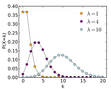
Which distribution increasingly approximates the sample mean as the sample size increases to infinity?
Let us suppose we have population data where the data are distributed Poisson
(see the figure for an example of a Poisson random variable).
Which distribution increasingly approximates the sample mean as the sample size increases to infinity?
The Central Limit Theorem holds that for any distribution with finite mean and variance the sample mean will converge in distribution to the normal as sample size 
 .
.
The Central Limit Theorem holds that for any distribution with finite mean and variance the sample mean will converge in distribution to the normal as sample size
Compare your answer with the correct one above
In a particular library, there is a sign in the elevator that indicates a limit of  persons and a weight limit of
  . Assume an approximately normal distribution, that the average weight of students, faculty, and staff on campus is
  , and the standard deviation is
  .
.
If a random sample of  people is taken, what is the standard deviation of their weights?
In a particular library, there is a sign in the elevator that indicates a limit of 


If a random sample of 
This question deals with the Central Limit Theorem, which states that a random sample taken from a large population where the sampling distribution of sample averages is approximately normal has a standard deviation equal to the standard deviation of the population divided by the square root of the sample size. The information given allows us to apply the Central Limit Theorem as it satisfies the necessary characteristics of the sampling distribution/size. The standard deviation of the population is 27lbs, and the sample size is 36; therefore, the standard deviation of the 36-person random sample is  , which gives us 4.5lbs.
This question deals with the Central Limit Theorem, which states that a random sample taken from a large population where the sampling distribution of sample averages is approximately normal has a standard deviation equal to the standard deviation of the population divided by the square root of the sample size. The information given allows us to apply the Central Limit Theorem as it satisfies the necessary characteristics of the sampling distribution/size. The standard deviation of the population is 27lbs, and the sample size is 36; therefore, the standard deviation of the 36-person random sample is
Compare your answer with the correct one above
Cat owners spend an average of  per month on their pets, with a standard deviation of
  .
.
What is the probability that a randomly chosen cat owner spends more than  a month on their pet?
Cat owners spend an average of
What is the probability that a randomly chosen cat owner spends more than
First, draw the appropriate curve to represent the problem: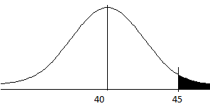
Because we want greater than 45, shade the right hand portion of the graph.
We will be using the z-distribution and not the t-distribution because we know the population standard deviation.
We will find the z-score for this cat owner, and then find the area to the right of that z-score to find the probability of spending more than $45.
We begin with the z-score formula:

Now find each value from the information given:


Fill in the formula


Now look this z-score up in the z-table to find the area under the curve. Look up 1.0 in the row and 0.00 in the column.
If your z table gives area shaded to the left, you will find
= 0.8413")
You want the area to the right, so subtract the above from 1.

If your z table gives area shaded to the right, you will find
= 0.1587")
Because you want the area to the right of z=1.0, this is your answer.
First, draw the appropriate curve to represent the problem:
Because we want greater than 45, shade the right hand portion of the graph.
We will be using the z-distribution and not the t-distribution because we know the population standard deviation.
We will find the z-score for this cat owner, and then find the area to the right of that z-score to find the probability of spending more than $45.
We begin with the z-score formula:
Now find each value from the information given:
Fill in the formula
Now look this z-score up in the z-table to find the area under the curve. Look up 1.0 in the row and 0.00 in the column.
If your z table gives area shaded to the left, you will find
You want the area to the right, so subtract the above from 1.
If your z table gives area shaded to the right, you will find
Because you want the area to the right of z=1.0, this is your answer.
Compare your answer with the correct one above
Cat owners spend an average of $40 per month on their pets, with a standard deviation of $5.
What is the probability that a randomly selected pet owner spends less than  a month on their pet?
Cat owners spend an average of $40 per month on their pets, with a standard deviation of $5.
What is the probability that a randomly selected pet owner spends less than
First, draw the distribution and the area you are interested in.
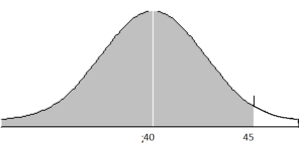
Next, calculate the z-score for the person of interest. Because the population standard deviation is known, we will use the formula for z-score and not t-score.
We will find the z-score for the person of interest, and then calculate the area under the curve that falls below, or to the left of that z-score.

Now we will find the value for each variable given in the problem:


Third, solve for z using the information in the problem.


Now we must determine the area under the curve to the left of a z-score of 1.0. We will consult a z-table.
Look up 1.0 in the row and 0.00 in the column.
If your z-table gives shaded area to the left, you will get
=0.8413")
We are interested in area to the left, which is what we found, so this is our answer.
If your z-table gives shaded area to the right, you will get
=0.1587")
Because we want the area to the left of z=1.0, we will subtract that area from 1:

First, draw the distribution and the area you are interested in.
Next, calculate the z-score for the person of interest. Because the population standard deviation is known, we will use the formula for z-score and not t-score.
We will find the z-score for the person of interest, and then calculate the area under the curve that falls below, or to the left of that z-score.
Now we will find the value for each variable given in the problem:
Third, solve for z using the information in the problem.
Now we must determine the area under the curve to the left of a z-score of 1.0. We will consult a z-table.
Look up 1.0 in the row and 0.00 in the column.
If your z-table gives shaded area to the left, you will get
We are interested in area to the left, which is what we found, so this is our answer.
If your z-table gives shaded area to the right, you will get
Because we want the area to the left of z=1.0, we will subtract that area from 1:
Compare your answer with the correct one above
It is known that cat owners spend an average of  a month on their pets, with a standard deviation of
  .
.
What is the probability that a randomly selected cat owner spends between  to
to  a month on their pet?
It is known that cat owners spend an average of
What is the probability that a randomly selected cat owner spends between
First, draw the distribution and the area you are interested in.
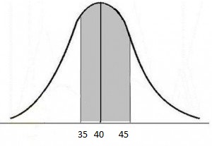
Next, we will need to calculate z-scores for both values we are interested in, and find the area under the curve that falls between these two values.
Because the population standard deviation is known, we will use the formula for z-score and not t-score.

We will find the z-score for the lower bound and find the z-score for the upper bound.
For the lower bound:


Now we will do the same for the upper bound:


Now we must determine the area under the curve which falls between z-scores of -1.0 and 1.0. To do this we will look up both z-scores and then subtract their areas (subtract the smaller area from the bigger area, so that you don't get a negative value).
For the lower bound, look up 1.0 in the row and 0.00 in the column. Then, for the upper bound, look up -1.0 in the row and 0.00 in the column.
The area to the left of 1.0 is 0.8413.
The area to the left of -1.0 is 0.1587.
To find the area between the two z-scores just subtract:

The central limit theorem states that the area under the curve + or - 1 standard deviation from the mean is 68.3%, which we have confirmed.
First, draw the distribution and the area you are interested in.
Next, we will need to calculate z-scores for both values we are interested in, and find the area under the curve that falls between these two values.
Because the population standard deviation is known, we will use the formula for z-score and not t-score.
We will find the z-score for the lower bound and find the z-score for the upper bound.
For the lower bound:
Now we will do the same for the upper bound:
Now we must determine the area under the curve which falls between z-scores of -1.0 and 1.0. To do this we will look up both z-scores and then subtract their areas (subtract the smaller area from the bigger area, so that you don't get a negative value).
For the lower bound, look up 1.0 in the row and 0.00 in the column. Then, for the upper bound, look up -1.0 in the row and 0.00 in the column.
The area to the left of 1.0 is 0.8413.
The area to the left of -1.0 is 0.1587.
To find the area between the two z-scores just subtract:
The central limit theorem states that the area under the curve + or - 1 standard deviation from the mean is 68.3%, which we have confirmed.
Compare your answer with the correct one above
If the Central Limit Theorem applies, we can infer that:
If the Central Limit Theorem applies, we can infer that:
The Central Limit Theorem tells us that when the theorem applies, the sampling distribution will be approximately normally distributed.
The Central Limit Theorem tells us that when the theorem applies, the sampling distribution will be approximately normally distributed.
Compare your answer with the correct one above